Party and Candidate Votes

This article offers a detailed analysis of the party_votes and candidate_votes datasets in the scgElectionsNZ package, shedding light on the voting dynamics in New Zealand’s elections.

Overview

The party_votes and candidate_votes datasets provide comprehensive insights into party preferences and candidate popularity across electorates. These datasets are pivotal for understanding how New Zealand’s Mixed-Member Proportional (MMP) system translates individual and party preferences into electoral outcomes.

Loading the Data

Begin by loading the party_votes and candidate_votes datasets to understand their structure and the information they contain:

Party Votes

# Load data
party_df <- scgUtils::get_data("party_votes")

# View data
head(party_df, 10)

Election	Ballot	Electorate	Party	Votes
2023	Party	Auckland Central	ACT Party	3301
2023	Party	Auckland Central	Animal Justice Party	50
2023	Party	Auckland Central	Aotearoa Legalise Cannabis Party	142
2023	Party	Auckland Central	DemocracyNZ	32
2023	Party	Auckland Central	Freedoms NZ	48
2023	Party	Auckland Central	Green Party	8503
2023	Party	Auckland Central	Informal	85
2023	Party	Auckland Central	Labour Party	8028
2023	Party	Auckland Central	Leighton Baker Party	3
2023	Party	Auckland Central	Maori Party	563

Candidate Votes

# Load data
candidate_df <- scgUtils::get_data("candidate_votes")

# View data
head(candidate_df, 10)

Election	Ballot	Electorate	Party	Votes	Percentage
2023	Candidate	Auckland Central	ACT Party	1235	3.59
2023	Candidate	Auckland Central	Green Party	16624	48.26
2023	Candidate	Auckland Central	Labour Party	2608	7.57
2023	Candidate	Auckland Central	National Party	12728	36.95
2023	Candidate	Auckland Central	NZ First	0	0.00
2023	Candidate	Auckland Central	Maori Party	0	0.00
2023	Candidate	Auckland Central	Other	1252	3.63
2023	Candidate	Banks Peninsula	ACT Party	2073	4.24
2023	Candidate	Banks Peninsula	Green Party	8325	17.03
2023	Candidate	Banks Peninsula	Labour Party	17464	35.72

As you can see, the candidate_votes dataset places all unsuccessful parties into “Other” and does not include Informal votes.

Combining Party and Candidate Vote Data

Amend Data

To resolve this issue, use the update_names() function to amend the party names:

# Amend Party names
party_df <- update_names(party_df) # default output = "party"

party_df <- party_df %>%
  filter(Party != "Informal") %>% # Remove "Informals"
  # Get grouped sum of Votes (i.e., combine all "Other" votes into one):
  group_by(Election, Electorate, Ballot, Party) %>%
  summarise(Votes = sum(Votes), .groups = 'drop') %>%
  ungroup() %>%
  # Get grouped percentage and round to 2 decimal places:
  group_by(Election, Electorate, Ballot) %>%
  mutate(Percentage = Votes / sum(Votes) * 100) %>%
  ungroup()

# View amended data
head(party_df, 10)

Election	Electorate	Ballot	Party	Votes	Percentage
2023	Auckland Central	Party	ACT Party	3301	9.33
2023	Auckland Central	Party	Green Party	8503	24.03
2023	Auckland Central	Party	Labour Party	8028	22.69
2023	Auckland Central	Party	Maori Party	563	1.59
2023	Auckland Central	Party	NZ First	1351	3.82
2023	Auckland Central	Party	National Party	11751	33.22
2023	Auckland Central	Party	Other	1881	5.32
2023	Banks Peninsula	Party	ACT Party	3919	7.91
2023	Banks Peninsula	Party	Green Party	9763	19.70
2023	Banks Peninsula	Party	Labour Party	13200	26.63

Merge Data

Then, combine both datasets for a unified analysis:

# Combine the two data frames
combined_df <- rbind(party_df, candidate_df)

Reshaping the Data

Reshape the data to understand how party and candidate preferences align or diverge:

combined_df <- combined_df %>%
  filter(Election == 2023) %>% # Get the 2023 election only
  # NB Ballot is amended to ensure that there are not two "Party" columns when pivoting wider:
  mutate(Ballot = ifelse(Ballot == "Party", "Party Vote", "Candidate Vote")) %>%
  select(Election, Ballot, Electorate, Party, Percentage) %>% # Remove Votes column
  tidyr::pivot_wider(names_from = Ballot, values_from = Percentage) # Pivot wider

# Make NAs = 0
combined_df[is.na(combined_df)] <- 0

# View data
head(combined_df, 10)

Election	Electorate	Party	Party Vote	Candidate Vote
2023	Auckland Central	ACT Party	9.33	3.59
2023	Auckland Central	Green Party	24.03	48.26
2023	Auckland Central	Labour Party	22.69	7.57
2023	Auckland Central	Maori Party	1.59	0.00
2023	Auckland Central	NZ First	3.82	0.00
2023	Auckland Central	National Party	33.22	36.95
2023	Auckland Central	Other	5.32	3.63
2023	Banks Peninsula	ACT Party	7.91	4.24
2023	Banks Peninsula	Green Party	19.70	17.03
2023	Banks Peninsula	Labour Party	26.63	35.72

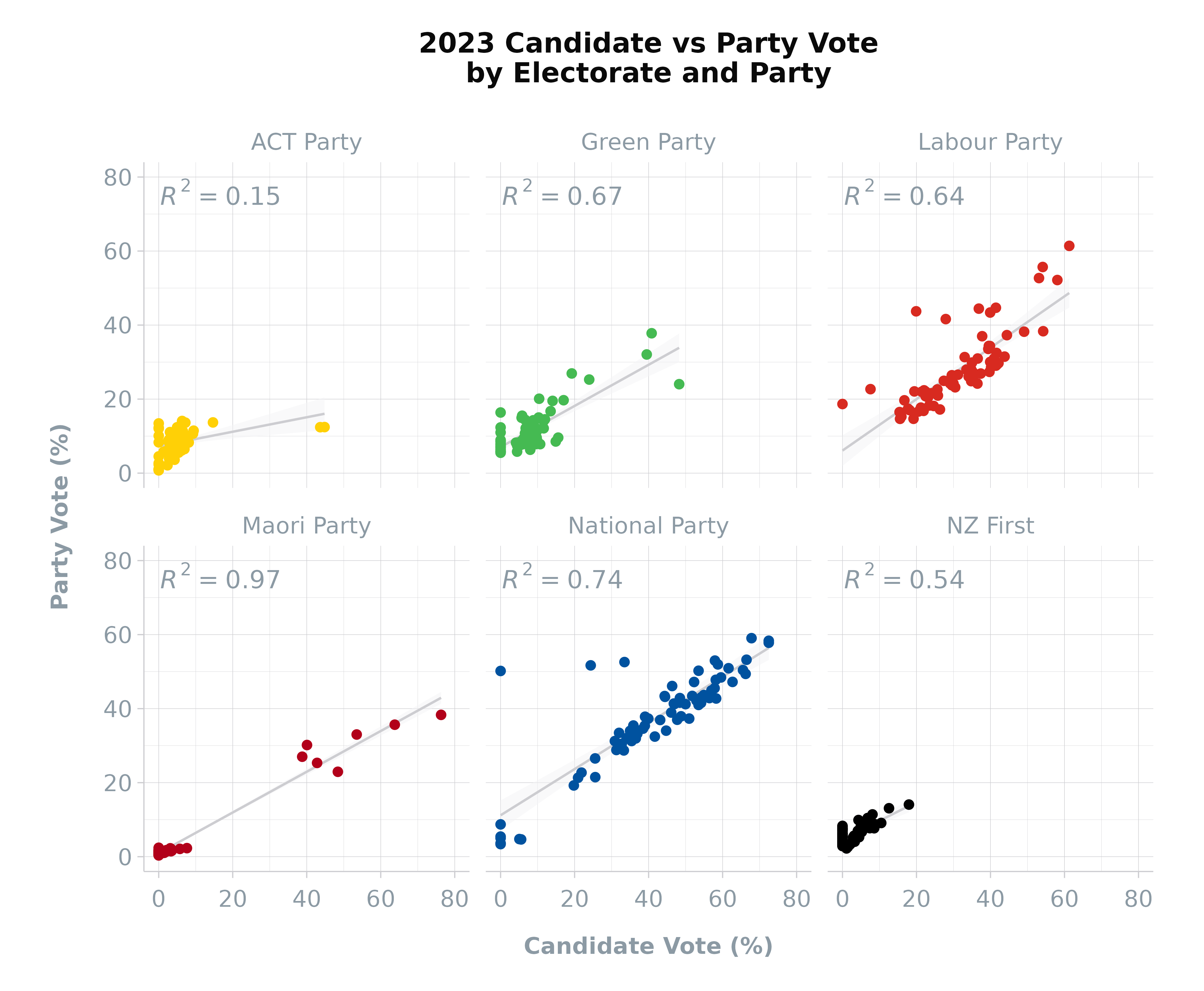
Visualising Party and Candidate Votes

Create a visualisation comparing Party and Candidate votes to understand the correlation between these two types of votes, which can indicate the degree of split voting by electorate. The colour_pal() function from the scgUtils package can be used to assign the party colours and the theme_scg() function from the same package can be used to customise the plot’s appearance:

combined_df %>%
  filter(Party != "Other") %>% # Remove "Other"
  ggplot(aes(x = `Candidate Vote`, y = `Party Vote`, colour = Party)) +
  geom_smooth(method = "lm", se = TRUE, formula = y ~ x, # Add linear regression
              colour = scgUtils::colour_pal("French Grey"),
              linewidth = 0.5, fill = "#F4F4F5", alpha = 0.5) +
  geom_point(na.rm = TRUE) + # Add scatter plot
  ggpmisc::stat_poly_eq(colour = scgUtils::colour_pal("Regent Grey")) + # Add R^2
  facet_wrap(. ~ Party) + # Facet by Party
  scale_colour_manual(values = scgUtils::colour_pal("polNZ")) + # Get party colours
  coord_equal(ylim = c(0, 80), xlim = c(0, 80)) + # Make axes equal
  labs(title = "2023 Candidate vs Party Vote\nby Electorate and Party", # Add labels
       y = "Party Vote (%)\n",
       x = "Candidate Vote (%)") +
  scgUtils::theme_scg() + # Apply theme
  theme(legend.position = "none") # Turn off legend